Linear Regression in Go - Part 3

Fri, Dec 4, 2015 |

In the previous posts we talked about how to predict a continuous value using a linear function and a way to measure the error given a matrix of test data and an hypothesis set of values theta.

In this post we’re describing a function that will converge the vector theta to its optimal values (or local miminum) which is called gradient descent.

Just to keep things simple, let’s assume we have a vector $\theta$ with just 2 dimensions (slope and intercept values of a simple line). If we plot the graph of $\theta_1$ , $\theta_2$ and the result of the cost function we’ll have something like:

Cost Function Graph

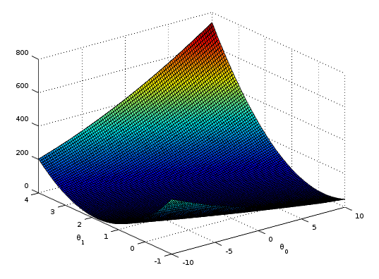
Given any random starting point $\langle\theta_0,\theta_1\rangle$ if we calculate the partial derivative of the function we’ll have a direction pointing away from the local minimum, so we can move a step closer ( $\alpha$ ) toward the opposite direction. This is our gradient descent in mathematical terms:

$$\theta_j := \theta_j - \alpha \frac{\partial}{\partial \theta_j} J(\theta_0, \theta_1)$$

The step we take every iteration toward the local minimum $\alpha$ is called learning rate (or sometimes step size ). For now let’s assume we use a fixed value and the same is for the numer of iterations we need to perform in order to get to the local minimum.

Deriving this formula results in the following:

$$\begin{align*} \text{repeat until convergence: } \lbrace & \newline \theta_0 := & \theta_0 - \alpha \frac{1}{m} \sum\limits_{i=1}^{m}(h_\theta(x_{i}) - y_{i}) \newline \theta_1 := & \theta_1 - \alpha \frac{1}{m} \sum\limits_{i=1}^{m}\left((h_\theta(x_{i}) - y_{i}) x_{i}\right) \newline \rbrace& \end{align*}$$

or in a more general way (if we assume $x_0^n=1$ ):

$$\begin{align*} & \text{repeat until convergence:} \; \lbrace \newline \; & \theta_j := \theta_j - \alpha \frac{1}{m} \sum\limits_{i=1}^{m} (h_\theta(x^{(i)}) - y^{(i)}) \cdot x_j^{(i)} \; & \text{for j := 0..n} \newline \rbrace \end{align*}$$

But what we want to implement is a vectorized version of that formula, which is:

$$\theta := \theta - \frac{\alpha}{m} X^{T} (X\theta - \vec{y})$$

Again, using vectors the result is much more readable and easier to implement. We can finally get to our actual go implementation:

 1// m = Number of Training Examples
 2// n = Number of Features
 3m, n := X.Dims()
 4h := mat64.NewVector(m, nil)
 5new_theta := mat64.NewVector(n, nil)
 6
 7for i := 0; i < numIters; i++ {
 8        h.MulVec(X, new_theta)
 9        for el := 0; el < m; el++ {
10            val := (h.At(el, 0) - y.At(el, 0)) / float64(m)
11            h.SetVec(el, val)
12        }
13        partials.MulVec(X.T(), h)
14
15        // Update theta values
16        for el := 0; el < n; el++ {
17            new_val := new_theta.At(el, 0) - (alpha * partials.At(el, 0))
18            new_theta.SetVec(el, new_val)
19        }
20}

h is a ~~Dense Matrix~~ Vector and numIters is a constant int64. You can find the full implementation here , and tests here .

A good visual explanation is in the following video by prof. Alexander Ihler :

Edit (feb 6 2016): I’ve fixed the code so now h and new_theta are of type Vector instead of DenseMatrix.